Elijah Whittle — Analytics

NBA Analytics

NBA
ANALYTICS

"Every game leaves a trace. This is how you read it."

Shot Chart Generator

Victor Wembanyama · 2025–26

Victor Wembanyama

2025–26 · San Antonio Spurs

—

FGA

—

FGM

—

FG%

—

3PA

—

3PM

—

3P%

—

Est. Points

Made

Missed

3PT

Fig 01 — Select a game above to animate Wembanyama's shot attempts on a real NBA half-court. Data via NBA Stats API. Orange filled = made · Ring = missed · Hover any dot for shot details.

Where does he score from?

The shot chart doesn't just show makes and misses. It shows the geometry of a player's game — the zones they dominate, the spots they avoid, the corners where they're quietly more efficient than anyone mentions. With Wembanyama, the shape is unlike any player the league has seen: rim finishes, corner threes, and pull-up threes from step-back range coexist in a single season profile. Every dot is a decision. The pattern is the player.

Wembanyama's post-All-Star shot profile shifts measurably — more above-break threes, fewer mid-range attempts. The chart makes that evolution visible without a single word of commentary.

ML Career Score Model

Who is closest to who?

Each dot is a player positioned by their career score — a composite metric from my ML model. Hover to explore. Click any dot to see who they're statistically closest to.

Fig 02 — Career Score Comparison. Scores computed by ML model trained on per-game stats, games played, and award history. Click any dot to animate nearest neighbors.

The model produces a single number that collapses a career into something comparable. It's not perfect — no number is — but when you click a player and see who slides toward them, you're seeing the model's opinion about statistical kinship. Sometimes it confirms what everyone knows. Sometimes it surprises you.

The score doesn't just reflect points. It weights longevity, awards, and multi-dimensional production. A player with 1,500 games at 17 PPG can score higher than a 30-PPG star who only played 600 games.

View in Colab GitHub

Next project

Machine Learning

MACHINE
LEARNING

"Can a stat line be predicted before it happens?"

The problem

Can a player's counting stats — points, rebounds, assists — be predicted from recent form and matchup context alone? This model treats each player-game as a forecasting problem: given how someone has played over their last 5 and 10 games, and who they're about to face, what should we expect next?

Architecture

From game log to forecast

RandomForestRegressor max_depth = 4 TimeSeriesSplit

01

Game Logs

Player game logs pulled from Basketball-Reference for stability across a full season.

02

Rolling Form

5-game and 10-game averages and volatility computed for every target stat.

03

Usage Proxy

Minutes, shot attempts and free throw rate approximate offensive involvement.

04

Matchup Adjust

What the opponent typically allows at each stat, layered in as matchup-adjusted features.

05

Random Forest

Standardized and encoded features feed a depth-limited ensemble regressor.

Fig 01 — Feature pipeline. Each stage feeds the next, and nothing downstream ever sees a game the model has not already passed.

Not just form — form against someone

Rolling averages and volatility (5-game and 10-game windows) are computed for every target stat, alongside minutes, shot attempts, and free throw rate. A simplified usage metric approximates each player's offensive involvement.

Opponent context — what a given team typically allows at each stat — is layered in to produce matchup-adjusted features: not just "how has this player performed," but "how has this player performed relative to what this opponent gives up."

Python scikit-learn pandas NumPy Random Forest

Built so it can't fool itself

A scikit-learn pipeline handles preprocessing — standardization for numeric features, one-hot encoding for categorical ones — feeding into a Random Forest Regressor, tuned conservatively (max depth of 4) to avoid overfitting on noisy per-game data.

Training uses a strict time-series split: the model only ever trains on past games and validates on future ones, avoiding the lookahead bias that sinks a lot of naive sports models.

No shuffling, no random splits. If the model can't predict a game using only what happened before it, the result doesn't count.

View on GitHub

Evaluation

Held to a forward-only backtest

Every prediction below was made before the game was played and graded against what actually happened, stat by stat, based on how close the forecast landed to the real result.

Read-out

Fig 02 — Average prediction accuracy by stat, based on how close each forecast landed to the actual result.

Fit

How closely predictions track reality

Each stat is plotted on its own scale — pooling points with three-pointers would manufacture a correlation that isn't there. The diagonal is a perfect prediction; the tighter the cloud hugs it, the better the model read that stat.

Hover any point to see the prediction behind it.

Fig 03 — Predicted vs. actual, by stat. r is the Pearson correlation within that stat. Points is the smallest sample and should be read with that in mind.

A note on R²

R² expresses how much of the variance in an outcome a model accounts for — an R² of 0.7 means roughly 70% of the game-to-game variation is explained. In live sports that is a brutally high bar. A single player's output swings on shot luck, foul trouble, blowout minutes, rotation changes and in-game matchup switches, and most of that is invisible to any feature set built from prior box scores.

Measured against one player's own variance over a handful of validation games, R² can read negative even when the predictions land close in absolute terms — the denominator is simply too small for the metric to behave. That is why this model is judged on the thing that survives that problem: how tightly its predictions track what actually happened, stat by stat.

Picking the right yardstick is part of the modelling work. A number that flatters the model but doesn't describe the problem isn't evidence of anything.

Case by case

Every prediction, player by player

The full graded record — strong runs and weak ones alike. Select a player to see every prediction the model made on them.

Fig 04 — Complete backtest log. Players ordered by sample size.

The spread between players is the honest part. Some profiles the model reads well — stable minutes, consistent role, predictable volume. Others it reads badly, and those tend to be the players whose usage swings with matchup or whose minutes move with foul trouble. Knowing which is which is the useful output, more than any single accuracy number.

Next project

Formula One Analytics

F—1

"The stopwatch captures everything. These tools are how we listen to it."

Fig 01 — Miami GP · Track Animation. Racing line and sector progression through the Miami International Autodrome, built from FastF1 telemetry data.

Multi-Driver Telemetry

LEC · STR · PIA — Race Fastest Laps

LEC STR PIA

RACE

DRIVERS

CHANNEL

TIME—

LEC—

STR—

PIA—

LEAD—

Fig 02 — Canada / Jeddah / Miami 2025 · Race fastest laps for Leclerc, Stroll, and Piastri. Speed, throttle, and brake channels extracted via FastF1. Scrub the timeline or hover to compare drivers at any point on the lap.

Where on the track does the gap actually open up?

A two-second gap at the flag looks like one thing in the standings and a completely different thing in the data. The Lap Time Analyzer pulls real race telemetry via FastF1 and breaks every lap into sectors — showing not just who was faster, but at which corner, on which lap, under which tire compound the delta grew.

Sector 2 deltas often reveal more than overall lap time. It's where setup decisions, brake bias, and driver commitment intersect — the invisible part of the race.

Fastest Lap Comparison (Teammates)

ANT vs RUS · Miami 2026 · Same car, different lap

ANT RUS

CHANNEL

ANT faster RUS faster

TIME—

ANT—

RUS—

Δ—

Fig 02 — Teammate fastest lap comparison · Miami 2026 · Speed channel. Green fill = ANT carrying more speed · Red fill = RUS carrying more speed. Hover or scrub to explore every moment of the lap.

Same car. What does the data reveal?

The teammate comparison is the cleanest experiment in motorsport — same machinery, same strategy, different driver. The Driver vs. Teammate Tool neutralizes the car advantage and isolates individual pace across qualifying and race stints.

When one driver is consistently 0.3s faster through the high-speed complex and 0.1s slower under braking, that's not noise. That's a skill profile.

Controlling for car performance is the key move. Without it, you're comparing driver talent plus machinery — which tells you nothing about either.

FastF1 pandas matplotlib Bokeh NumPy

View on GitHub

Next project

Computer Vision

COMPUTER
VISION

"Seeing is easy. Understanding is built."

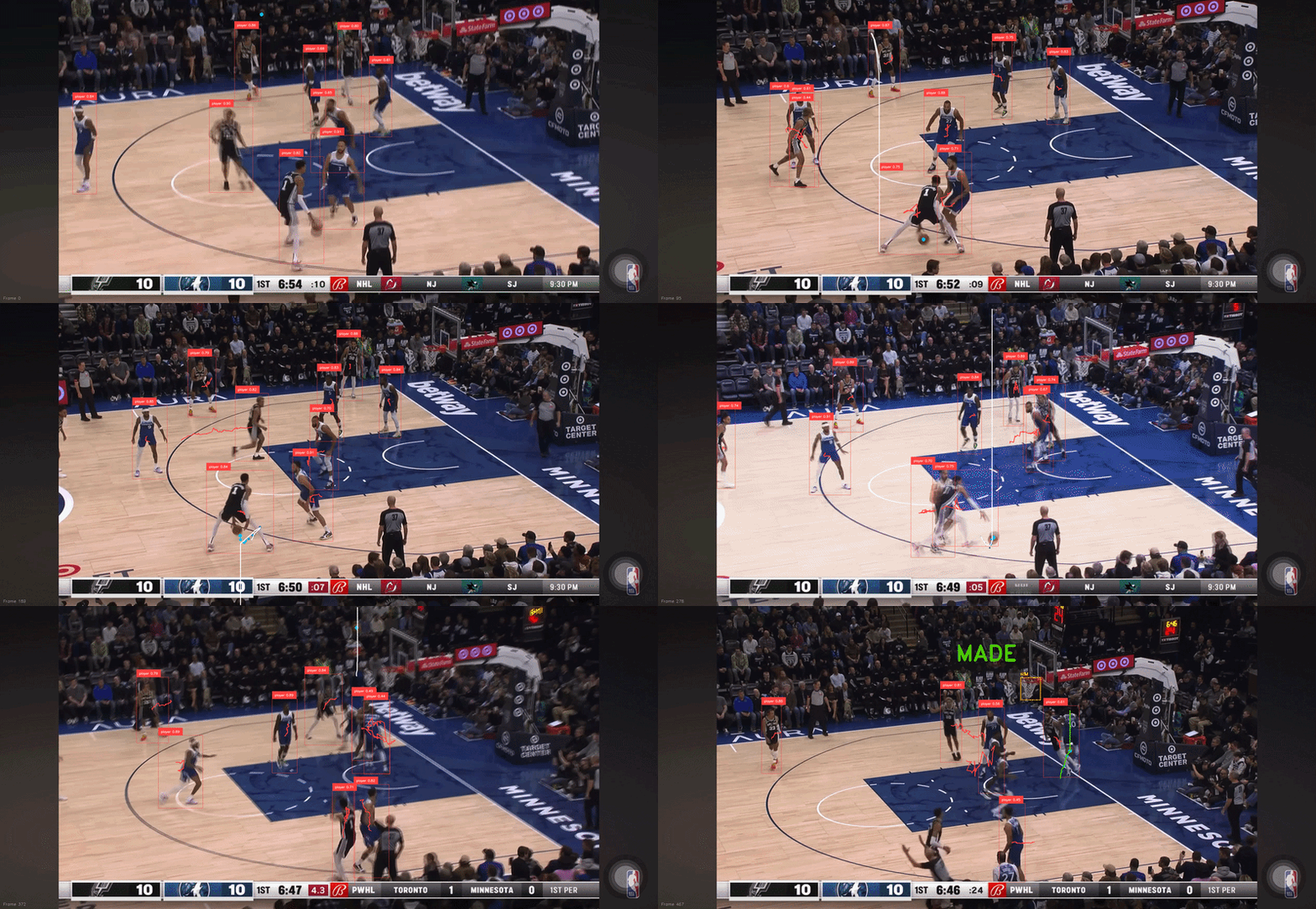
Fig 01 — Wembanyama Step-Back · Model Output. Trajectory overlay computed frame by frame: ball detection, arc path, release angle, and peak annotated in real time. OpenCV + custom tracking pipeline · 59 fps.

Can a model trace the exact arc of a Wembanyama step-back?

This pipeline applies computer vision to one of the most unguardable shots in the NBA — Wembanyama's step-back jumper. Frame by frame, it extracts ball position, calculates trajectory, and annotates the flight path with release angle and arc data. The output makes visible what broadcast angles obscure: the precise geometry that makes this shot so hard to contest.

Trajectory modeling at the player level turns broadcast footage into measurement data — the same kind that coaching staffs pay millions to collect manually.

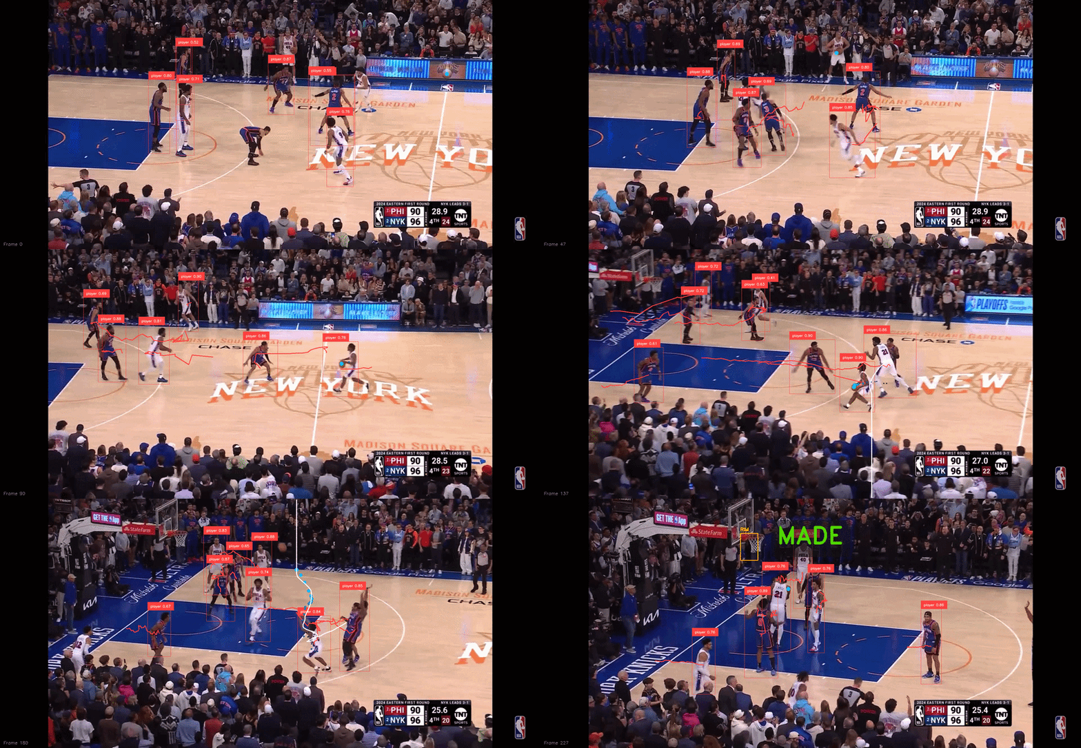
Tracking Tyrese Maxey — one of the fastest players alive

Applied YOLO detection and SORT tracking to Tyrese Maxey footage, locking a persistent bounding box onto him through contact, screens, and full-speed cuts. At Maxey's pace, maintaining ID integrity across frames is a genuine technical challenge — one that pure detection models fail under pressure.

The annotated output logs position and proximity to other tracked players on every frame — the raw material for automated spacing and off-ball movement analysis that no box score captures.

When the tracker holds lock at 40+ mph cutting speed without re-assigning IDs, the model is generalizing — not memorizing camera angles.

YOLO SORT DeepSORT OpenCV Python

View on GitHub

ELIJAH
WHITTLE

CS student, data scientist, live sports broadcaster — in that order, depending on the day.

The goal

Driven by a fierce passion for competition, my goal is to join a forward-thinking sports organization where relentless preparation and data drive competitive edge. I focus on turning raw datasets into applicable tactical advantage. Building computer vision tracking tools, predictive models, and custom data workflows that directly inform decision-making. Through hands-on sports analytics projects and coursework in algorithms, computer science, and statistics, I combine deep technical precision with a high-stakes competitive mindset to help teams win.

"The data already knows what the game is trying to say. The tool is just how you listen."

Relevant coursework

MATH & STATISTICS

Calculus I & II Linear Algebra Discrete Math Probability & Statistics

MACHINE LEARNING & ALGORITHMS

Machine Learning Analysis of Algorithms

PROGRAMMING & SYSTEMS

Data Structures Advanced OOP Computer Networks Software Engineering Database Systems Design

Tools

Python scikit-learn pandas OpenCV YOLO R Bokeh SQL C++

Experience

Live Event Operator — EDGIO

September 2020 – June 2025 · Remote

Collaborates with major national sports broadcasters on live programming delivery. Manages software tools for live transitions, ensuring minimal downtime under real broadcast pressure. Front-row seat to how sports media actually operates.

Research Intern — Foul Territory

September 2025 – Present · Remote

Built the MLB analytics pipeline behind Foul Territory's broadcast rundowns, including a recurring Gameday Research deliverable — storylines, clinch scenarios, and pitching matchups that hosts reference live on air.

Education

University of the District of Columbia

B.S. Computer Science · Expected 2027 · GPA 3.5

Get in touch

Open to work, collaborations, and conversations about sports data.

whittle.elijah@gmail.com GitHub LinkedIn

Back to start

MLB Analytics

MLB

This scouting lab breaks down hitter performance using Statcast data. Use the zone grid to see where a player makes contact, the EV histogram to assess bat speed, and the stats table to compare month-to-month trends. Higher barrel% and hard-hit% indicate quality contact.

Batted Ball Profile

Pitch Speed vs Exit Velocity · Click a point

Exit Velo —

Launch Angle —

Distance —

Pitch Type —

Pitch Speed —

Contact —

Fig 01 — Statcast batted ball data · 2D: pitch speed vs exit velocity (red shading = 95+ mph hard contact) and launch-angle profile · 3D: every batted ball plotted as its own physics parabola from contact through flight, coloured by contact type · Click a point to view velocities/angle · Filter by pitch type or contact result above.

What does his arsenal look like?

Hitting is only half the matchup. A pitcher's identity lives in where the ball leaves his hand and how it moves on the way to the plate. Release point reveals arm slot and repeatability — a tight cluster means a delivery a hitter can't read pitch-to-pitch. Movement separates the arsenal: which offerings ride, which sweep, which drop off the table. Together they explain why the same velocity plays completely differently from two different arms.

Elite arms disguise their pitches by releasing everything from the same tunnel, then letting movement do the work in the final feet. The release chart shows the disguise; the break chart shows the payoff.

Pitch Arsenal

Release Point & Movement · Click a pitch

Velocity —

Spin Rate —

Pitch Type —

H-Break —

V-Break —

Fig 02 — Statcast pitch data · 2D: release point (catcher POV) and horizontal vs vertical break (in) · 3D: every pitch drawn as a curved trajectory from release to plate, with break driving the curvature · Click a pitch to inspect velo, spin and movement · Filter by pitch type or result above.

Continue to